The Ascape Model Developer’s Manual
Section 3.
The Ascape Tutorial
Section 1. Agent-based Modeling
Section 2. The Ascape Modeling Framework
Section 3. The Ascape Tutorial
3.1 The Coordination Game Model
3.1.1 Finishing the CoordinationGame Class
3.1.1.2 Creating all of the agents
3.1.2 Making the CoordinationGamePlayer Class
3.1.2.2 The CoordinationGamePlayer Class
3.1.4 Adding Statistical Operations
3.2 Experimenting with the Model
3.2.1 Editing Model Properties at Runtime
3.2.2 Adding Stochasticity to Model
3.2.3 Adding Averaging Statistics to the Model
3.2.5 A Biological Coordination Game
3.2.6 Dynamic Neighborhoods and Social Networks
In the last part of Section 2, we built the basic framework for a Coordination Game model. In what follows, we will flesh out that framework to make a working model, and then we will expand on that model to illustrate some of Ascape’s more interesting functionalities.
The model we have created so far is below. The Java operator for commenting code (//), will be used throughout the code samples to add annotations.
public class CoordinationGame extends Scape {
//These three integer variables define the dimensions of the
//lattice and the number of agents in the model
public int nPlayers = 200;
public int latticeWidth = 30;
public int latticeHeight = 30;
//These two instance variables will be this model’s scape graph
//and it’s players scape.
Scape lattice;
Scape players;
//The ‘createScape’ method constructs the scapes for the model, specifies the //agents and execution order, and adds the scapes to the model.
public void createScape() {
//first we call the constructor for the Scape class
super.createScape();
//next we create the 2Dlattice with a von Neumann neighborhood //structure, set its prototypical agents, and set its dimensions
lattice = new Scape(new Array2DVonNeumann());
lattice.setPrototypeAgent(new HostCell());
lattice.setExtent(latticeWidth, latticeHeight);
//then we create an instance of the CoordinationGamePlayer class so //that we can assign it to the lattice and make it
//the prototype agent for the players scape.
CoordinationGamePlayer cgplayer = new CoordinationGamePlayer();
cgplayer.setHostScape(lattice);
//then we create the players scape, set the prototype agent, and set //the execution order.
players = new Scape();
players.setPrototypeAgent(cgplayer);
players.setExecutionOrder(Scape.RULE_ORDER);
//finally, we add the specified scape graph and the
//specified players scape to the model.
add(lattice);
add(players);
}
}
In order to build a working Ascape model, we need to expand this basic framework to include some key functionalities that have not been discussed. Section 2 outlined the basic conceptual structure of a model. This part of section 3 covers some technical aspects to constructing an Ascape model that have less to do with conceptual architecture and more to do with details of implementation.
Finishing the CoordinationGame Class
When we create a scape graph, it takes on all the properties of a CA, but it is not yet a ‘graphical’ component of the model. The scape graph is a mathematical object: it is an N x N lattice populated with cell agents. Once we add the lattice to the model, the Java engine stores all of its information but the engine does not know how to draw the lattice so that we can watch it run. Thus, if we were to run the above model, it would calculate the outcome, but we would not be able to see it. In order to make the model visible, we need to create a view object and add it to the scape graph. Statistical operations, which we will handle below, are managed similarily; in order to collect statistics on a model, we need to create a statistics view and add it the appropriate scape.
There are numerous view objects that come standard with Ascape. Of course, you can always extend one of these classes to write your own. The standard view most often used to show the scape graph is the basic, 2D overhead view. This view simply represents the scape graph as a 2D lattice with the (0, 0) coordinate (origin) in the top, left corner. This view object is called the Overhead2DView.
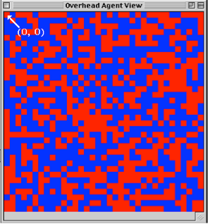
Fig. 24: Overhead2Dview
There is also an overhead 2D view that allows the developer to relativize the origin of the lattice to any coordinate on the graph. This is called OverheadRelative2DView.
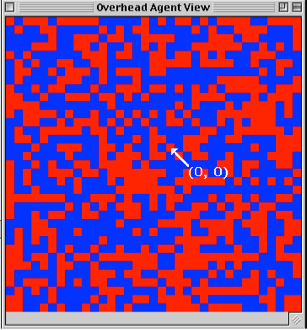
Fig. 25: OverheadRelative2DView
In some Ascape models, agents do not interact on a spatial graph. For example, in the Firms model, every agent is located in a 1D list that is divided up into smaller collections, called firms. There is no spatial component to this model, since all interactions occur between agents simply based on their membership in a 1D list, and not on their location in it. In this model, there are no neighborhoods, but only amorphous collections of agents. In the Retirement model, agents are located on a 2D scape graph, but their significant interactions happen through network relations. In both of these models, simply showing an overhead 2D view would be meaningless. So, they employ views that show the relevant 1D data. In the Retirement model, the entire players list is shown horizontally, and the agents are colored by their properties (retired or not). This horizontal array scrolls to show the new state of the players list at each time step. This is called a Scrolling1DView.
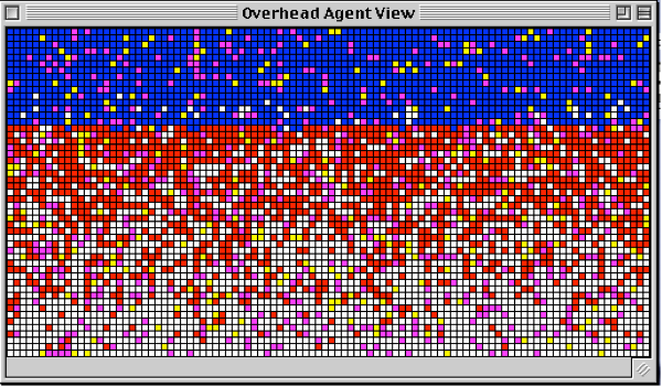
Fig.26: Scrolling1Dview (Retirement model)
The Firms model does not use a lattice at all. In the Firms model, agents switch firms by moving from sub-list to sub-list (or “firm to firm”) within the main players list. The view object for this model simply displays a vertical list of the firms (sub-lists), showing the number of agents in each firm list. This view object, called the FixedStretchyView, allows the developer to easily visualize comparisons in the sizes of sub-lists.
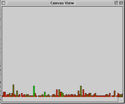
Fig.27: Fixed Stretchy View
The Coordination Game Model is a fairly basic spatial game on a 2D lattice, so we will use the basic Overhead2DView class. The first thing to do is to add a variable to the CoordinationGame Class that can hold the new view object. This variable will be of type Overhead2DView because it will hold an instance of the Overhead2DView class.
public class CoordinationGame extends Scape {
public int nPlayers = 200;
public int latticeWidth = 30;
public int latticeHeight = 30;
Scape lattice;
Scape players;
//This is the view object variable that will hold our instance of the //Overhead2DView class
Overhead2DView view;
.
.
.
}
The vertical ellipses in the code examples:
.
.
.
will be used to avoid redundancy of code that is inessential to the example.
Next, we will create a method called createGraphicViews(), in which we construct the view and add it to the scape graph. We do not need explicitly to call the createGraphicViews() method. Like createScape(), createGraphicViews() is automatically called on startup.
public void createGraphicViews() {
//call the basic view setup for a Scape List
super.createGraphicViews();
//Create the new view
overheadView = new Overhead2DView();
//Set its cell size to, say, 15
overheadView.setCellSize(15);
//add the view to the scape graph.
lattice.addView(overheadView);
}
In the createGraphicViews() method, we first call the Scape class’s createGraphicViews() method. This insures that any general setup routines defined in the superclass will be performed. We then create the new Overhead2Dview with the ‘view’ variable, and then we set the cell size. Setting the cell size does not affect the dynamics of the model at all, but simply determines how much of the screen the model will occupy. Finally, we add the new view object to the scape graph. View objects should be thought of as windows into a scape. They attach to the scapes to present representations of their agent population. Some view objects attach to scape graphs, other view objects (such as charts) can attach to other kinds of scapes. But, in general, the purpose of a view object is to visualize the contents of a scape. Once we add the ‘overheadView’ object to the lattice, we have created a window into the scape graph.
In setting up the model, we must tell the players scape how many of the cgplayer agents we want to have. We have already created an integer variable ‘nPlayers’, to which we assigned the value ‘200’. Now, we need to used that value to tell the players scape how many agents to add to itself. We do this with the Like CreateScape() and Creategraphicviews(), public void scapeSetup(ScapeEvent scapeEvent) is called automatically when the model launches.
public void scapeSetup(ScapeEvent scapeEvent) {
((Scape) players).setExtent(new Coordinate1DDiscrete(nPlayers));
}
The onSetup() method tells the ‘players’ scape to set its size to fit an array of nPlayers, which, in this case, is 200. Since cgplayer was assigned as the prototypical agent for the ‘players’ scape, this scape now has 200 agents of type cgplayer.
The basic structure of the working model is now complete. It looks as follows:
public class CoordinationGame extends Scape {
//create variables
public int nPlayers = 200;
public int latticeWidth = 30;
public int latticeHeight = 30;
Scape lattice;
Scape players;
Overhead2DView overheadView;
//create scapes and create agents
public void createScape() {
super.createScape();
lattice = new Scape(new Array2DVonNeumann()); lattice.setPrototypeAgent(new HostCell());
lattice.setExtent(new Coordinate2DDiscrete(latticeWidth, latticeHeight));
CoordinationGamePlayer cgplayer = new CoordinationGamePlayer();
cgplayer.setHostScape(lattice);
players = new Scape();
players.setPrototypeAgent(cgplayer);
players.setExecutionOrder(Scape.RULE_ORDER);
add(lattice);
add(players);
}
//create views
public void createGraphicViews() {
super.createGraphicViews();
view = new Overhead2DView();
overheadView.setCellSize(15);
lattice.addView(overheadView);
}
//populate the model with agents
public void onSetup() {
((Scape) players).setExtent(new Coordinate1DDiscrete(nPlayers));
}
}
So, with these four steps we have
This model is ready to run except for the small problem that the class CoordinationGamePlayer does not exist. Once we create this class, we will be able to fill the ‘players’ scape with cgplayer agents, and run the model.
Making the Coordination Game Player Class
The coordination game agent is very basic. It simply looks around in its local neighborhood (which has been defined by the lattice as a von Neumann neighborhood), and picks a random neighbor to play. The payoff matrix looks as follows.
Red Blue
Red1, 1 0, 0
--------------
Blue 0, 0 1, 1
Fig. 28: Coordination Game Payoff Matrix
In this coordination game, the agents are trying to coordinate on color. Each round, agents either get a 0 for failing to coordinate, or a 1 for coordinating. Next, we need to choose a mechanism for how the players will decide what color to play. They could play a best reply, or they could play imitation, or they could play some more complicated version of a rational choice strategy. To start, we will make the agents very dumb and have them be simple imitation agents. These agents look around the neighborhood for the agent who has scored the highest on its five most recent plays, and they imitate the color of that agent.
So, the properties of the cgplayer agent are as follows. It has:
So, the agents only need to have:
To create the CoordinationGamePlayer class, first we setup the variables and initialize the class.
public class CoordinationGamePlayer extends Cell Occupant{
//create our variables
protected Color myColor;
protected int totalScore;
protected int[] recentPlays;
//we also add a variable so we can keep track of the first five plays.
protected int count = 0;
public void initialize() {
if (randomInRange (0,1) > 0)
{
myColor = Color.red;
}
else
{
myColor = Color.blue;
}
recentPlays = new int [5];
}
}
As discussed in Section 2, the CoordinationGamePlayer agent is a cell occupant agent, so it must extend the class CellOccupant. The initialize() method is called automatically when each new agent is created. This method assigns either red or blue to the agent, with a probability of .5. It also creates the ‘recentPlays’ array with a length of 5.
In order for the variable ‘myColor’ to effect the color of the agent when it is rendered on the screen, we must have a method getColor() that can be called by the system. This method is also useful so that other agents can find out what color an agent is.
Public Color getColor(){
Return myColor;
}
Now that we have created and initialized our variables, we need to make some rules for the agents.
In Ascape, rules are not attached to individual agents but to the scapes in which they are located. Intuitively, every agent in the ‘players’ scape will have the same set of rules (e.g., imitate the most successful player in the neighborhood, find a partner and play, etc.). This list of rules executes across all active players in the scape. In addition to efficiency, a benefit of having the scape own the rules for the agents is that it gives the user the ability to change the rules at runtime. Scape-level properties can be edited in the Settings window while the model is running. This allows the user to change the order of the rules, to make the rules execute in AGENT-ORDER, or RULE-ORDER (i.e., asynchronously or synchronously), and to eliminate some rules from the agent’s behavior, all without having to change the code.
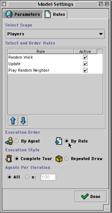
Fig.29: Settings window (Rules Tab) in Running Model
This is a basic concept in Ascape programming: designing scape-level properties modularly, so that we can experiment on the population of agents without having to rewrite the agent code each time.
For convenience, Ascape is designed so that these scape-level rules can be added from within the class that defines the agent. This allows us to inspect the agent and its Of course, these rules do not, in point of fact, belong to the agent, but to the scape in which the agent is located. When the agent class (CoordinationGamePlayer) is first created, the model will call the class’s ScapeCreated() method. This method is used to add rules directly to the agent’s parent scape (in this case, the ‘players’ scape).
public void scapeCreated() {
getScape().addInitialRule(MOVE_RANDOM_LOCATION_RULE);
getScape().addRule(RANDOM_WALK_RULE);
getScape().addRule(UPDATE_RULE);
getScape().addRule(PLAY_RANDOM_NEIGHBOR_RULE);
}
First, we are going to add an initial rule, which is executed only on setup. This rule tells the scape to place the agents on random locations on the lattice. Then we will add three behavioral rules, which will be executed by the scape on every iteration of the model. An iteration of the model is simply an execution of the Root Scape’s singe ITERATE rule. This rule activates all of the Root Scape’s agents (the scape graph and the ‘players’ scape), and causes their rule sets to fire. The first rule for the ‘players’ scape simply tells the agents to move to a new, neighboring cell every turn. The agents are, in essence, doing a random walk each turn. We do not need to write any additional code for this rule. The UPDATE_RULE is an empty placeholder that calls an update() method, which we need to write. We will use the UPDATE rule as the search for the best player in the neighborhood. The PLAY_RANDOM_NEIGHBOR_RULE automatically finds a random cell occupant in the lattice neighborhood, and returns this agent to a play() method. It is up to us to write this play() method. Our play() method will take the agent that it is passed, play the coordination game with it, and then add the result to our ‘recentPlays’ array and update the ‘totalScore’ variable.
By default, the rules will be executed in the order that they are listed. This can be changed at runtime from the Settings window. For now, however, we assume that agents will initially be placed randomly, and that every iteration they will first move to a new location, then evaluate which of their neighbors to imitate, and then play the coordination game. The agents’ evaluations of which neighbor to imitate will be triggered by the UPDATE_RULE, which automatically calls the update() method. So, we need to write an update() method that finds the best-scoring agent in the neighborhood, and imitates that agent.
public void update() {
count++;
if (count > recentPlays.length)
{
int currScore = 0;
int bestScore = this.totalScore;
List neighbors = findNeighborsOnHost();
for (Object neighbor : neighbors) {
{
currScore = ((CoordinationGamePlayer)neighbors[i]).totalScore;
if (currScore > bestScore)
{
bestScore = currScore;
myColor = ((CoordinationGamePlayer)neighbors[i]).getColor();
}
}
}
}
First notice that this method only runs its evaluation of the neighborhood if the agent has played more than five times. This is to ensure that the value of ‘totalScore’ accurately reflects a full ‘recentPlays’ array. Thus, agents do not start imitating other agents until everyone’s totalScore reflects five plays of the coordination game. An important note is that this way of writing the model assumes that the entire ‘players’ scape is iterated through on every turn. This is the normal procedure for a model, however we can change this procedure so that agents are chosen by random draw, or so that only a subset of the agent population is activated during an iteration of the model. Using these latter two procedures, it is not a correct assumption that just because this agent has played five times (count > 5), that all of his neighbors have played five times. However, for now, we can safely assume that all agents will be activated on each iteration, which means that if this agent’s totalScore reflects at least five plays, then so does the totalScore of his neighbors.
The agent looks around his neighborhood using the findNeighborsOnHost(); method. So, the full command first gets the host cell directly below the agent (getHostCell()), and then tells that host cell to get the neighboring occupants. The neighborhood that is surveyed is, of course, defined by the scape graph. In this case, it is a von Neumann neighborhood. The findNeighborsOnHost() call returns a list of cell occupants. We put them into an array called ‘neighbors’, and then iterate through the array looking for the highest value of the ‘totalScore’ variable. Note that the array is a CellOccupant array by default. In order to reference the ‘totalScore’ variable, we have to cast the contents of the array to be CoordinationGamePlayer. In summary, the agent does an uphill search on its neighbors’ values for 'totalScore', and imitates the highest scoring agent in the neighborhood. Of course, the agent only changes its color if the best totalScore in the neighborhood is higher than its own.
public void play(Agent partner) {
int score;
if (((CoordinationGamePlayer)partner).getColor() == myColor)
{
score = 1;
}
else
{
score = 0;
}
updateRecentPlays(score);
}
public void updateRecentPlays(int score){
totalScore = 0;
for (int i = 0; i < (recentPlays.length - 1); i++){
recentPlays[i] = recentPlays [i + 1];
totalScore = totalScore + recentPlays[i];
}
recentPlays[recentPlays.length - 1] = score;
totalScore = totalScore + recentPlays[recentPlays.length - 1];
}
The play() method is called by the PLAY_RANDOM_NEIGHBOR_RULE, and it takes an agent as an argument. This method simply assigns the player a score of one for coordinating with the partner agent, or a score of zero for failing to coordinate. It then calls the updateRecentPlays() method, to add the new score to the ‘recentPlays’ array and to update the value of the ‘totalScore’ variable.
The CoordinationGamePlayer Class
All told, the CoordinationGamePlayer class looks as follows:
public class CoordinationGamePlayer extends CellOccupant {
//create variables
protected Color myColor;
protected int totalScore;
protected int[] recentPlays;
protected int count = 0;
//initialize the variables for each new agent
public void initialize() {
if (randomInRange (0,1) > 0)
{
myColor = Color.red;
}
else
{
myColor = Color.blue;
}
recentPlays = new int [5];
}
//create the list of rules for scape
public void scapeCreated() {
getScape().addInitialRule(MOVE_RANDOM_LOCATION_RULE);
getScape().addRule(RANDOM_WALK_RULE);
getScape().addRule(UPDATE_RULE);
getScape().addRule(PLAY_RANDOM_NEIGHBOR_RULE);
}
//specify the UPDATE_RULE: imitate the most successful neighbor
public void update() {
count++;
if (count > recentPlays.length)
{
int currScore = 0;
int bestScore = this.totalScore;
List neighbors = findNeighborsOnHost();
for (Object neighbor : neighbors) {
currScore = ((CoordinationGamePlayer)neighbors[i]).totalScore;
if (currScore > bestScore)
{
bestScore = currScore;
myColor = ((CoordinationGamePlayer)neighbors[i]).getColor();
}
}
}
}
//specify PLAY_RANDOM_NEIGHBORS_RULE: 1 for coordinating, 0 for not
coordinating. Then update the records.
public void play(Agent partner) {
int score;
if (((CoordinationGamePlayer)partner).getColor() == myColor)
{
score = 1;
}
else
{
score = 0;
}
updateRecentPlays(score);
}
// Update the record of wins, and the totalScore
public void updateRecentPlays(int score){
totalScore = 0;
for (int i = 0; i < (recentPlays.length - 1); i++){
recentPlays[i] = recentPlays [i + 1];
totalScore = totalScore + recentPlays[i];
}
recentPlays[recentPlays.length - 1] = score;
totalScore = totalScore + recentPlays[recentPlays.length - 1];
}
//Standard getColor method
public Color getColor() {
return myColor;
}
}
The CoordinationGame class combined with the CoordinationGamePlayer class define a complete Ascape Coordination Game Model.
So, in summary :
To create the model class:
To create the agents class:
You will notice that the payoff matrix for this coordination game is completely symmetrical. A user of the model may wonder what would happen if we changed the payoffs so that coordinating on red gave a reward of 2, while coordinating on blue only gave a reward of 1. In the current design of the model, we must change the code inside the agent class in order to run this experiment. As we saw above, properties of the scapes (e.g., the rules) are accessible to the user through the Settings window. Additionally, properties of the model (model-scope variables) are also available for the user to edit through the Settings window. The nPlayers variable, the lattice_height variable, and the lattice_width variable can all be changed by the user at runtime. Similarly, we can create variables in the model class, say ‘coordinateOnBlue’ and ‘coordinateOnRed’, that the user can edit in the Settings window. Instead of hard-coding the payoffs into the agent class (as we did above), we can use these variables to determine the agents’ payoffs for coordinating on blue or red. Thus, the users can experiment with the dynamics of the model by changing the value of these variables at runtime. In fact, good coding practice for Ascape in general is to make important variables part of the model class. These variables can then both be accessed by the agents and edited by the user, giving the user dynamic control over the behavior of the agents.
In order for model variables to appear in the Settings window, and for the user’s changes to them to take effect in the model, the developer must write get() and set() methods for these variables. When the Settings window is opened it automatically looks for all available get() methods of model-scope variables and populates itself. Similarly, when changes are made in the Settings window, the set() method is automatically called to update the model while it runs. So, to add user control over the payoff matrix, we will first add our new variables to the model and then we will add the get() and set() methods.
public class CoordinationGame extends Scape {
public int nPlayers = 200;
public int latticeWidth = 30;
public int latticeHeight = 30;
//new variables for coordination on Red and Blue
public int coordinateOnBlue = 1;
public int coordinateOnRed = 1;
.
.
.
public int getRedScore(){
return coordinateOnRed;
}
public void setRedScore(int NewcoordinateOnRed){
coordinateOnRed = NewcoordinateOnRed;
}
public int getBlueScore(){
return coordinateOnBlue;
}
public void setBlueScore(int NewcoordinateOnBlue){
coordinateOnBlue = NewcoordinateOnBlue;
}
}
The method getRedScore() reports the value of the variable ‘coordinateOnRed’, allowing it to show up in the Settings window. The method setRedScore() changes the value of ‘coordinateOnRed’ to the value entered in the Settings window. setRedScore() is automatically called by the Settings window when the user edits the ‘RedScore’ variable. The model must have get() and set() methods for any variable that the developer wants the user to be able to edit from the parameters window.
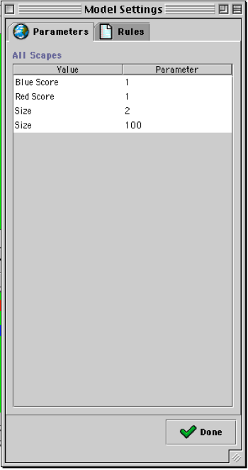
Fig.30: Parameters Window with new variables.
Now that the user can access these variables, the agents need to be able to access them, too.
public void play(Agent partner) {
int score;
if ((((CoordinationGamePlayer)partner).getColor() == myColor) && (myColor == Color.blue))
{
score = ((CoordinationGame)getRoot()).getBlueScore();
}
else if ((((CoordinationGamePlayer)partner).getColor() == myColor) && (myColor == Color.red)) {
score = ((CoordinationGame)getRoot()).getRedScore();
}
else
{
score = 0;
}
updateRecentPlays(score);
}
Notice that in order to reference the getRedScore() method, we need to call the getRoot() method, and then cast it to the CoordinationGame model. This call returns the Root Scape for the model, but it returns it as a Scape object, which must be cast to a CoordinationGame object in order to reference the desired get() method. This kind of casting procedure is fairly common in Ascape since the Ascape calls return basic data structures (such as Scapes) which need to be cast to the specific type of object that the developer is using (e.g., the CoordinationGame Scape).
In order to inspect an agent's properties when a model is running, you can ALT + click on the agent and an Agent Inspection window will appear. This window will display the agent's parameters with their current values. Just like in the model's Settings window, the variables that are displayed in the Agent Inspection window are the ones that have get() and set() methods for them. Analogously to the methods used to get and set model variables, get() and set() methods for agent variables are usually put at the end of the agent class. As a rule of thumb, it is useful to write get() and set() methods for most of your agent variables so that you can inspect them as the model is running. This is very helpful for debugging models.
Statistical operations are a useful way of gleaning information from the model. Like the views discussed above, statistical operations are windows into scapes. The difference in the case of the statistical operation is that instead of operating on just the scape graph, they operate on every kind of scape. In general, stats are added to scapes to provide detailed information about the properties of their members. To take a basic example from the Coordination Game Model, let us collect a statistic on the number of agents that are red and blue at any given time. This statistical operation is window into the ‘players’ scape. All of the code for the statistical operations is within the createScape() method.
public void createScape() {
...
StatCollector CountReds = new StatCollectorCond("Reds") {
public boolean meetsCondition(Object object) {
return (((CoordinationGamePlayer) object).myColor == Color.red);
}
};
StatCollector CountBlues = new StatCollectorCond("Blues") {
public boolean meetsCondition(Object object) {
return (((CoordinationGamePlayer) object).myColor == Color.blue);
}
};
players.addStatCollector(CountReds);
players.addStatCollector(CountBlues);
}
First, we create the objects that will hold the statistics. One is called ‘CountReds’, the other is called ‘CountBlues’. In order to make these objects, we need to specify a kind of statistical operation. In this case, we use a simple conditional statistical operation, called StatCollectorCond: if an object in the scape meets the condition (i.e., returns ‘true’), then it is included in the statistic. In this case, the condition is that the object is a certain color. The first statistical operation counts all of the red agents, and the second one counts all of the blue agents. Once these operations are defined, they are added to the players scape.
When the model runs, it will perform the ‘CountReds’ and ‘CountBlues’ operations every iteration. In order to see these stats, we need to add a chart to the model; a chart is a window that displays statistics. There are two ways to do this. First, one can create a chart at run time, using the Ascape Toolbar to select the chart dialog box. The user can then select whether to view the stats as a time series, a histogram, or a pie chart. Also, the user can dynamically assign colors to the stats.
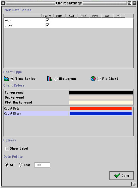
Fig.31: Creating a chart at runtime.
This is the easiest way to add a chart to the model in which to view the statistics that you have created. However, if you create your chart this way, it goes away when the model closes. These ‘runtime’ charts need to be created using the dialog box every time the model is opened. If you want a chart to launch with the model, you can specify all of the same information that is in the dialog box in the content of the createGraphicViews() method. This will create a new chart window and fill it with your stats when the model launches. Of course, the content of this window can also be edited at runtime from the chart dialog box.
To add a chart to the model this way, we need to create a chart, add the stats, and specify the plotting dimensions.
public void createGraphicViews() {
.
.
.
ChartView chart = new ChartView();
players.addView(chart);
chart.addSeries("Count Reds", Color.red);
chart.addSeries("Count Blues", Color.blue);
chart.setDisplayPoints(100);
}
First, we create a new chart and add it to the ‘players’ scape. Then we add each of the stats to the chart. The stats can be graphed in a number of ways, but we are choosing to graph them as a time series. So, we use the chart.addSeries() method. The first argument to this method gives both the operation being performed (Count) and the name of the stat (Reds) in a single string. We use a string, instead of two arguments, so that this parameter can be used as the label for this series on the chart. So, the “Count Reds” label, will be attached to a time series that graphs the count (number of players) that satisfy the “Reds” statistical operation. The second argument tells the chart to use the color red to chart this series. Similarly, we do the same for the “Blues” stat. Finally, we set the dimensions of the chart to show 100 iterations, or time steps, along the horizontal axis.
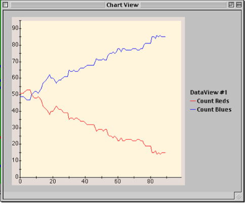
Fig.32: Chart View with new statistics
We are now finished writing the Coordination Game Model. In the next part of the tutorial, we will see how Ascape allows us to experiment with the model by changing / adding parameters, adding statistics, and changing the agent dynamics. See the Appendix 1 for the complete source code of the model.
Editing Model Properties at Runtime
We have already seen that we can change a scape’s rules, and a model’s parameters at runtime. But, we can also change whether a scape executes its rule synchronously or asynchronously, and whether a scape iterates through all of its agents, or picks random agents on every iteration of the model. These parameters can all be set from within the Ascape code, but they can also be edited on the fly in the Settings window.
All of the properties listed in the rules tab are relevant to the scape that is selected in the ‘Select Scape’ menu at the top of the window. In the base case, there are three scapes that one can choose from: the Root Scape (i.e., the Model), the Scape Graph (e.g., 2D lattice), and whatever scape contains the agents (e.g., Players). If there are more scapes, or sub-scapes, these will appear in the list as well.
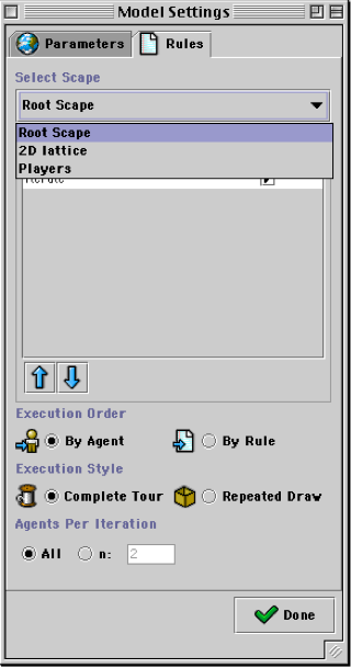
Fig.33: Settings Window (pull down of scapes)
Once a scape is chosen, the ‘Select and Order Rules’ panel will display all of the rules that are part of the scape. They are displayed in the order in which they are executed. Each rule can be checked or unchecked (making it active or inactive in the current run of the model). And, if a rule is selected, it can be moved earlier or later in the execution order by clicking on the up and down arrows.
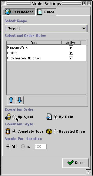
Fig.34: Settings window (editing rule order)
The ‘Execution Order’ radio buttons allow the user to select whether the model will run synchronously or asynchronously. Intuitively, the ‘By Agent’ option is asynchronous, and the ‘By Rule’ option is synchronous. The ‘Execution Style’ radio buttons determine whether the scape iterates through all of its members every iteration, or whether it picks random agents. In the latter case, it may well happen that during an iteration of the model some agents are randomly chosen more than once, and some agents are not chosen at all. Finally, the ‘Agents per Iteration’ radio buttons determine how many of a scape’s agents it iterates through during one step of the model. If the players scape is selected, then it can either activate ‘All’ of its members (i.e., 100), or it can activate some number between 0 and 100.
In base case for the Coordination Game Model, the 2D lattice scape does not have any agents, so its setting is irrelevant. The Root Scape has 2 agents: the 2D lattice scape and the players scape. By default the Root Scape only has 1 rule: ITERATE. This rule simple tells the scape to activate each of its sub-scapes. Since the Root Scape only has one rule, it is irrelevant whether it is set to execute in Agent Order or in Rule Order. In either case, the 2D lattice and the ‘players’ scape will both be activated in the same way. The Execution style for the Root Scape should always be Complete Tour, otherwise an entire scape of agents could be omitted from an iteration of the model. And, for similar reasons, the Agents Per Iteration is generally set to ‘All’.
The Players scape has three rules, and we can mix their order, or turn them off. But, for now, we will experiment with the other scape settings. We coded the players scape to execute in RULE_ORDER. By default it will execute a complete tour of all the agents. This default setting ensures that all agents will be activated during each iteration of the model. However, if ‘Agents Per Iteration’ is set to ‘n: 50’, ‘Execution Style’ is set to Repeated Draw, and ‘Execution Order’ is set to ‘By Agent’. Then instead of iterating through each rule for each agent, the model with pick a random agent, iterate through all of its rules, and then pick another agent (possibly that same agent again). Since we set ‘Agents Per Iteration’ to 50, the model will pick 50 times, and then start a new iteration. But, you can easily see that we quickly lose the significance of the end of one iteration and the beginning of another. Since the only scape, besides the Root Scape, with active agents is the players scape, the model runs like a continuous random selection of agents (making the ‘Agents Per Iteration’ parameter essentially irrelevant).
Try experimenting with the model under these conditions, notice that the model still converges, but takes much longer to do so. For any model, it is important to test its behavior under conditions of synchronous / asynchronous updating, and complete tour / repeated draw. They are important tests for robustness and model validation. Similarly, activating/deactivating and changing the order of rules at runtime can be a useful way of experimenting with the dynamics of complex models in which multiple scapes have agents with multiple rules.
Adding Stochasticity to the Model
Now that we have seen some of the ways that we can experiment with the behavior of the Coordination Game Model, we can begin to expand on the model by adding more interesting behavior to the agents. One easy way to do this is to introduce some stochasticity into the model. In the current model, agents always choose to imitate the color that is the most successful in their neighborhood. Although this makes sense, we may wonder what would happen if we added some noise to this decision-making process – so that 10% of the time agents would choose randomly. We can run this experiment by adding a variable to the model called ‘error’. Then we say that with the probability of ‘error’, an agent will not choose to imitate the best in the neighborhood, but will choose its color randomly. We will make ‘error’ a model-scope variable, so that we can edit it from the Settings window and see how the model behaves under different error rates.
First, we add the variable ‘error’ to the CoordinationGame class, with get() and set() methods so we can access it from the Settings window.
public class CoordinationGame extends Scape {
protected int nPlayers = 100;
protected int latticeWidth = 30;
protected int latticeHeight = 30;
public int coordinateOnBlue = 1;
public int coordinateOnRed = 1;
//new variable
public int error = 0;
Scape lattice;
Scape agents;
Overhead2DView overheadView;
.
.
.
//get and set methods
public int getError(){
return error;
}
public void setError(int NewError){
error = NewError;
}
}
Next, we change the update() rule in the CoordinationGamePlayer class to include the possibility of error. The error variable determines the percentage of the time that the agent will choose randomly instead of imitating the best in the neighborhood.
public void update() {
count++;
if (count > recentPlays.length)
{
//if the random number between 1 and 100 is greater than, or
//equal to ‘error’, proceed as normal
if (randomInRange(0,100) >= ((CoordinationGame)getRoot()).error)
{
int currScore = 0;
int bestScore = this.totalScore;
List neighbors = findNeighborsOnHost();
for (Object neighbor : neighbors) {
currScore = neighbor.totalScore;
if (currScore > bestScore)
{
bestScore = currScore;
myColor = ((CoordinationGamePlayer)neighbors[i]).getColor();
}
}
}
//otherwise, choose randomly
else
{
if (randomInRange (0,1) > 0)
{
myColor = Color.red;
}
{
myColor = Color.blue;
}
}
}
}
Error is initially set to 0, but we can open the Settings window and change it to, say, 10. If we wait until the model converges, and then change the ‘error’ value, we see about ten percent of the population jump out of convergence.
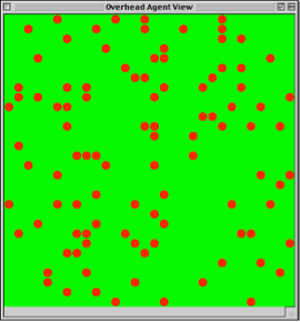
Fig.35: Model converging
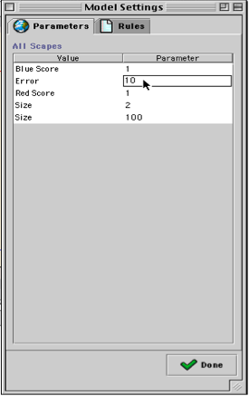
Fig.36: Settings window (introducing error)
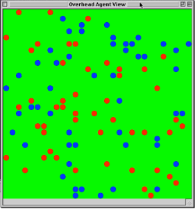
Fig.37: Model ‘shocked’ with error
Once we ‘shock’ the model with an error rate greater than 0, we can reset the value of error to 0, and watch to see if the model switches equilibria and converges to a different color. We can experiment with population sizes and error rates to see what value of error is needed to ‘bump’ a model from one equilibrium to another.
Also, instead of changing the error rate back to 0 once the model has been shocked, we can leave the error at the new rate. If we run the model this way, the population will never converge, and it will simply exhibit a pattern of noisy interactions. An interesting experiment to run at this point is to change the payoff matrix so that it is asymmetrical. With the Settings window already open, we can simply change, say, the value of RedScore from 1 to 2. Now, the model should quickly converge on all red. However, if we keep a constant error rate in the model, we should always see a small population of blue agents. At this point, the model will show a ‘stochastically stable’ heterogeneous population of agents. The ratio of reds to blues will depend on the payoff matrix and the error rate, but we can see that simply by adding error, the simple coordination game shows a complex, but stable, pattern of agent behavior.
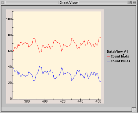
Fig.38: Asymmetrical Payoffs with Constant Error
Adding Averaging Statistics to the Model
Now that we have added a bit more complexity to the model, we may be interested in how this affects the payoffs of the agents. In the case where error = 0 and payoffs are symmetric, we know that the model will converge so that everyone will receive the same payoff of 1 every turn. We may wonder, however, whether in the case where error = 10 and red payoff = 2, whether the society has higher overall welfare or lower overall welfare than the base case. Because of the increased payoff for red coordination, the red agents will certainly have a higher welfare than any of the agents in the base model. However, because of the frequent errors, many agents will also receive a 0 payoff for miscoordination. So, we many want a new statistic that will tell us the overall welfare of the society, so that we can compare the model with error and asymmetric payoffs to the model with no error and symmetric payoffs.
To add the new statistic to the CoordinationGame class, we follow the same coding pattern used earlier, but this time we will not use the StatCollectorCond Stat Collector class, because we do not have a condition that needs to be satisfied. Rather, we want to collect data from every agent, and then to average this data over the total number of agents. To do this, we use the StatCollectorCSAMM class, which allows us to perform averaging operations on the data it collects. So, we go the createGraphicViews() method in the CoordinationGame class.
public void createGraphicViews(){
.
.
.
//create stat collector that will get payoff information
StatCollector AvgPayoff = new StatCollectorCSAMM("Payoff") {
public double getValue(Object object) {
return ((CoordinationGamePlayer) object).getRunningTotal();
}
};
.
.
.
//add stat collector to the players scape
players.addStatCollector(AvgPayoff);
//add average payoff series to the chart
chart.addSeries("Average Payoff", Color.black);
}
First, we create the stat collector ‘AvgPayoff’, using the class StatCollectorCSAMM. We label this statistic “Payoff”. The method getValue() calls the getRunningTotal() method inside CoordinationGamePlayer, which will return the totalScore variable that each CoordinationGamePlayer agent has. This is a standard get() method, like the ones used above, which we will need to add to the CoordinationGamePlayer class. It will allow us to retrieve each agent’s totalScore so that they can be summed and averaged by the StatCollectorCSAMM class. Once the statistic is created, we add it to the ‘players’ scape. We can add this statistic to the chart already created in the createGraphicViews() method or to a chart at runtime using the chart dialog box. We will add it in the code so that all three statistics appear when the model opens. We add it to the chart as time series that performs an averaging operation (i.e., we call it “Average Payoff”). Once we add the getRunningTotal() method to the CoordinationGamePlayer class, we can watch this stat run.
public class CoordinationGamePlayer extends Cell Occupant{
.
.
.
public int getRunningTotal(){
return (totalScore * 10);
}
}
The getRunningTotal() method returns the ‘totalScore’ variable multiplied by 10. We use this increased magnitude simply to make small fluctuations in the average value of ‘totalScore’ visible in the time series. Intuitively, the base model will converge to one color, and the ‘totalScore’ variable will converge to 5 (since there is a memory that is 5 plays long, and every play, after convergence, should produce a 1 for everyone). This will display on the chart as a line at the value 50.
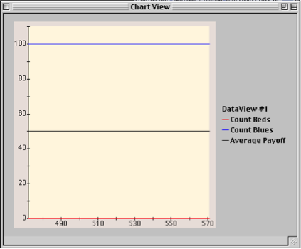
Fig.39: Base Model with Payoff graph.
If we add error to the model, and increase the red payoff, we see that the average payoff spikes and then fluctuates around 75. So, in the main, social welfare is higher when there is a small degree of error and a high asymmetric payoff, than when there is no error and a low symmetric payoff.

Fig.40: Stochastic Model with Payoff Graph
This result seems consistent with our intuitions, but the graph is useful because it clearly shows how social welfare varies with changes in error rate and payoffs. So, now we can experiment with the parameter values to see how much error the higher payoff asymmetry can sustain before payoffs start to dip below the payoffs for the symmetric model. Significantly, all of these experiments can be made while the model is running (in the Settings window), without having to change any code.
The Coordination Game that we have been developing uses imitation as the basic behavioral rule. However, after we have experimented with this model, we may want to explore other rules for coordinating agents. A common one is best reply. Using a best reply rule, agents keep a record of their opponents’ strategies in previous plays, and then they decide what to play by determining what is a best reply to the majority of opponent strategies that they have encountered. In the symmetric payoff Coordination Game, the best reply is simply to play the same color that has made up the majority of an agent’s interactions. However, the expected payoff of a decision is the likelihood of an outcome (in this case, the frequency of a color in an agent’s history) times the payoff for that outcome. So, in an asymmetric game, we must factor the payoff matrix into the agent’s decision.
In order to make the Coordination Game Model into a best reply model, we must rewrite the update() method (the contents of the UPDATE rule), so that agents will use the history of their partners’ decisions to decide what color to play. So in addition to the ‘recentPlays’ array, we need a second array that will keep a record of the colors that the agents’ partners have played; let us call it the ‘recentPartners’ array. The update() method will walk through the ‘recentPartners’ array, find the frequency of red and the frequency of blue, and multiply these frequencies by the payoffs for coordinating on red and coordinating on blue. Whichever value is larger will be the color that the agent will play. At the start, these payoffs are both 1, so this last operation has no effect. However, we will build it into the model so that once we start experimenting with payoff parameters, the agents will be equipped to make the correct evaluations.
All the changes for the best reply model take place in the CoordinationGamePlayer class.
public class CoordinationGamePlayer extends CellOccupant {
protected Color myColor;
protected int totalScore;
protected int[] recentPlays;
protected int count = 0;
//add the partners array
protected Color[] recentPartners;
//add variables to hold the running totals of reds and blues in the //partners array
protected int totalreds;
protected int totalblues;
//we use the random choice algorithm three times in this class, so to keep
//things tidy, I have made it a separate method, called ‘doRandom()’
public void doRandom(){
if (randomInRange (0,1) > 0)
{
myColor = Color.red;
}
else
{
myColor = Color.blue;
}
}
//each time the agent plays, it updates the score array (recentPlays), and
//also updates the recentPlayers array.
public void play(Agent partner) {
.
.
.
updateRecentPlays(score);
updateRecentPartners(((CoordinationGamePlayer)partner).getColor());
}
//the agents update the recentPartners array with the color of the most
//recent player, and also keep a running total of red and blue partners
public void updateRecentPartners(Color ncolor){
totalreds = 0;
totalblues = 0;
for (int i = 0; i < (recentPartners.length - 1); i++){
recentPartners[i] = recentPartners [i + 1];
if (recentPartners[i] == Color.red)
{
totalreds = totalreds + 1;
}
else if (recentPartners[i] == Color.blue)
{
totalblues = totalblues + 1;
}
}
recentPartners[recentPartners.length - 1] = ncolor;
if (ncolor == Color.red)
{
totalreds = totalreds + 1;
}
if (ncolor == Color.blue)
{
totalblues = totalblues + 1;
}
}
//The update method is where the agent decides what to play. The agent //multiplies the number of reds in its recent history by the payoff for red //coordination, and the number of blues by the payoff for blue coordination. //Whichever number is largest determines the agent’s next play. If the
//values are tied, the agent chooses randomly. Also, I have left the error
//code in the update method, so that we have the option of experimenting with //errors in the best reply model.
public void update() {
count++;
if (count > recentPlays.length)
{
if (randomInRange(0,100) >= ((CoordinationGame)getRoot()).error)
{
int redScore;
int blueScore;
blueScore = totalblues * ((CoordinationGame)getRoot()).getBlueScore();
redScore = totalreds * ((CoordinationGame)getRoot()).getRedScore();
if (redScore > blueScore)
{
myColor = Color.red;
}
else if (blueScore > redScore)
{
myColor = Color.blue;
}
else
{
doRandom();
}
}
else
{
doRandom();
}
}
}
Since our agents will be ‘boundedly rational’ agents, the ‘recentPartners’ array should be relatively small. I have chosen to keep the ‘recentPlays’ array and the ‘recentPartners’ array to a length of 5. Experimenting with this value can also change the dynamics of the model. As above, we can also experiment with the best reply dynamics by making the ‘error’ variable positive, and by changing the payoff matrix.
A Biological Coordination Game
A different direction to take the Coordination Game Model is to eliminate decision making altogether and make it an evolutionary game theoretic model. To do this, we need to replace the imitate and best reply rules with reproduction and death rules. In the biological model, agents reproduce when their score gets to a certain value (say, 5), and then their score is reset to 0. As agents keep coordinating, they keep reproducing. Agents who fail to coordinate (e.g., who have a score of 3 or less after 5 turns) die off. While in the previous model, agents could change color based on their best options, in this model, agents are fixed as either blue or red, and the evolutionary dynamics determine which ‘genotype’ will survive.
To make the Coordination Game Model into a biological model, we will need to change the rule set for the ‘players’ scape. Players will no longer call an UPDATE rule to evaluate their best options. Rather, they will play, and then they will call a METABOLISM rule to determine whether they should reproduce or they should die. We will add a few new variables (e.g., ‘repScore’ and ‘minScore’) as constraints on reproduction and death. We will make these variables model-scope variables with get() and set() methods, so that we can experiment with different values for reproduction and death to see how they affect the dynamics of the model.
These changes to the Coordination Game Model primarily take place in the class CoordinationGamePlayer, except for the addition of new model-scope variables, which are added to the CoordinationGame class.
public class CoordinationGamePlayer extends CellOccupant {
.
.
.
//we remove the UPDATE rule, and add a METABOLISM rule, which calls the
//metabolism method, added below.
public void scapeCreated() {
getScape().addInitialRule(MOVE_RANDOM_LOCATION_RULE);
getScape().addRule(RANDOM_WALK_RULE);
getScape().addRule(PLAY_RANDOM_NEIGHBOR_RULE);
getScape().addRule(METABOLISM_RULE);
}
//The metabolism() method (called by the METABOLISM rule) evaluates on
//the totalScore variable. If totalScore equals ‘repScore’, then the
//agent reproduces. Initially, ‘repScore’ will be set to 5, but it can
//be changed in the Settings window.
public void metabolism(){
if (totalScore == ((CoordinationGame)getRoot()).getrepScore())
{
count = 0;
reproduce();
for (int i = 0; i < (recentPlays.length - 1); i++){
recentPlays[i] = 0;
}
}
//If the totalScore variable is less than the repScore, then the agent //evaluates whether it should die. If the agent’s total score is less than //the MinDieScore, and the agent has been through ‘TurnstoDie’ number of //turns, then the agent dies. Initially, the ‘MinDieScore’ is 3, and the //‘TurnstoDie’ is 5. So, if the agent is not successful in coordinating more //than 3/5 of the time, then it will die.
else if (totalScore <= ((CoordinationGame)getRoot()).getMinDieScore() && count >= ((CoordinationGame)getRoot()).getTurnstoDie())
{
this.die();
}
}
//To reproduce, the agent first makes sure that there is a neighboring spot
//where the baby can be placed. So, agent reproduction is constrained by the //density of the neighborhood. If there is a space, we create a new agent, //called ‘baby’, of type CoordinationGamePlayer. We add this agent to the //‘players’ scape, so that it will have all of the rules that are owned by
//the scape, and it will live on the ‘lattice’ scape graph. We initialize
//the new agent to set its basic properties, but then we explicitly set its
//color to match the parent’s color (because the initialize() method sets the //color randomly). Finally, we place the new, initialized agent onto the //lattice.
public void reproduce(){
if(this.getHostCell().isNeighborAvailable())
{
CoordinationGamePlayer baby = (CoordinationGamePlayer) this.clone();
((Scape) this.getScape()).add(baby);
baby.initialize();
baby.setColor(myColor);
baby.moveTo(this.getHostCell().findRandomAvailableNeighbor());
}
}
There are two final changes to CoordinationGamePlayer class. First, the reproduction() method calls a This is used to set the color of the baby to the color of the parent. We need to create this method.
public void setColor (Color NewColor){
MyColor = NewColor;
}
Second, since we are using the count variable to determine how many plays an agent has been through, we need to add a line of code to the play() method that increments ‘count’ every time the agent plays an opponent.
public void play (Agent partner){
.
.
.
count = count + 1;
}
Finally, we need to add our new model-scope variables to the CoordinationGame class, with get() and set() methods.
public class CoordinationGame extends Scape {
.
.
.
public int turns = 5;
public int repScore = 5;
public int minScore = 3;
.
.
.
public int getTurnstoDie(){
return turns;
}
public void setTurnstoDie(int Newnum){
turns = Newnum;
}
public int getrepScore(){
return repScore;
}
public void setrepScore(int Newscore){
repScore = Newscore;
}
public int getMinDieScore(){
return minScore;
}
public void setMinDieScore(int Newscore){
minScore = Newscore;
}
The biological version of the Coordination Game Model exhibits interesting spatial behavior. As agents successfully reproduce, they build dense neighborhoods of same-color neighbors. These neighborhoods rapidly spread until the entire lattice is covered with agents. The neighborhood that grows the fastest has more members, and so has more agents trying to reproduce. The border areas between the two neighborhoods are areas of ‘low fitness’, and these agents are constantly dying off. Since the larger group has more agents vying for reproductive space, its agents fill the border areas more quickly than the smaller group. Soon, the smaller group is run to extinction, and the population fixates on one color.
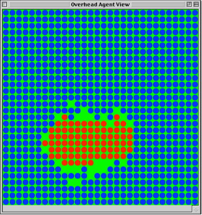
Fig.41: Biological Coordination Game Model
As in the previous versions of the Coordination Game Model, we have used model-scope variables so that the user can explore the dynamics of the model without having to edit the code. Also, the developer can easily add a few lines of code to introduce error into the reproduction process, essentially adding ‘mutation’ to the model.
Dynamic neighborhoods and social networks
Let us step back from the biological, or reproduction, version of the Coordination Game, and return to the earlier versions with decision theoretic agents. In those versions of the Coordination Game Model, all of the interactions were spatially localized. The PLAY_RANDOM_NEIGHBOR rule automatically uses the geometry of the scape graph to assign partners. Looked at from a networks perspective, using the model’s von Neumann geometry to assign playing partners is tantamount to creating a dynamic partners network. Also, using the local neighborhood as the basis for evaluating the best player to imitate creates a dynamic imitation network. These social networks overlapped because they were using the same Von Neumann neighborhood. The partners network and imitation network are both dynamic because the cgplayer agents are moving each turn, so that the actual members of the neighborhood changes every iteration of the model. As we have seen, using the local neighborhood to determine the contents of the partners network and the imitation network produces interesting consequences for the ‘demographics’ of the model.
The imitation model that we have written exhibits an interesting spatial pattern in the emergence of a dominant color. All of the agents coordinate locally. The coordinating neighborhoods spread until one neighborhood dominates the others. This kind of spatial pattern is also observed in the best reply and reproduction models. And, it is often a very good approximation of natural behavior. However, the underlying phenomenon in these models is the spatially constrained networks of interacting agents. When these networks are characterized by local neighborhoods, they exhibit spatially localized behavior patterns. However, networks of interactions can take many forms, and exhibit many kinds of patterns.
If, for example, we wanted to change the network structure of the best reply model so that agents were not playing their local neighbors, but rather could play any random agent in the model, we would only have to change one line of code. Instead of the PLAY_RANDOM_NEIGHBOR rule, we could use the PLAY_OTHER rule. This rule tells the agent to execute the Essentially, this change of rule turns a local interaction model into a global interaction model. The end result is the same, however the spatial pattern in the model is lost, and the model takes longer to converge. So, in this case the agent has a much more disperse, by still dynamic, network. Except in very abstract models, this network structure is generally undesirable because its behavioral analog is that agents can interact randomly with any member of the entire population at any time. This seems, in most cases, unlikely if not implausible.
A different, more plausible, social network structure is a network that is neither dynamic nor spatial. In such a network, we begin by assigning each agent a collection of agents that constitute its social network. These agents, however, are not the spatially related to one another. They can be randomly assigned, or assigned based on some other property (say, membership in a club or society). The point is that these agents interact with one another as part of a social network, even though they are not spatially related to one another. This kind of network highlights the fact that what is essential about the models that we have been looking at is how the network of agents is constituted. Spatial factors are often the most salient in the construction of dynamic social networks. However, networks of interacting agents will often be dispersed within a population. Further, agents will often have multiple sets of social networks for different kinds of interactions.
Using the basic coordination model as a starting point, we can construct an example of this new kind of social network model. It is one in which as agents move around, they keep a small, static network of ‘friends’ agents against whom they judge their success. They use this network to evaluate their strategies, and determine what color to adopt. At the same time, they play the coordination game in local neighborhoods. So, the local social networks determine the agents’ payoffs, while the static friends networks determine their behavior (color choice). While a well-scoring agent will dominate the strategies in a friends network, this dominance does not affect the choices of his game-playing network. Consequently, the reinforcement mechanism found in the original imitation model is not present, so neighborhoods do not show the same patterns of spatial coordination as in the earlier models. However, global coordination in the model is achieved more quickly precisely because there are no ‘neighborhood effects’, where pockets of reinforcement allow a minority population to keep imitating one another. The diffusiveness of social influence in this social network model allows the population to coordinate much more quickly, and dramatically.
To write this model, we begin by having each agent select four random agents to be part of its friends network. Once these agents are selected, they will always be the four agents that the agent uses to evaluate its strategy. As the model runs, the agents migrate to new neighborhoods, and play different agents, but they always refer to their friends network when deciding what color to play. In the model we will write, friends networks are not symmetric, which is to say that if A has B in its friends network, there is no guarantee that B has A in its network. We can change this later to make the social networks more tight-nit, but it seems intuitively plausible at the outset that people might imitate friends or acquaintances who will not imitate them.
To make the imitation Coordination Game Model into a friends-network model, the first thing to change is the initial setup. We need to create the social network when the model is created. To do this, we will add a rule to the scape that tells each agent in the scape to pick four random agents and to create a social network of these agents. This rule, like the MOVE_RANDOM_LOCATION_RULE, will only be called when the model is initialized, and so will be added to the scape using the addInitialRule() method. However, there is no existing rule for setting up social networks, so we will have to create a new rule.
public void scapeCreated() {
getScape().addInitialRule(MOVE_RANDOM_LOCATION_RULE);
getScape().addInitialRule(new Rule("SetNewNetwork")
{
public void execute(Agent agent) {
((CoordinationGamePlayer) agent).setNewNetwork();
}
});
getScape().addRule(RANDOM_WALK_RULE);
getScape().addRule(UPDATE_RULE);
getScape().addRule(PLAY_RANDOM_NEIGHBOR_RULE);
}
I have called the new rule “SetNewNetwork”. Creating a new rule simply involves creating an instance of the Rule class and writing an execute() method that takes an agent as an argument (overriding the existing execute() method in the In this case, the execute() method simply tells the agent to call its setNewNetwork() method. Now, to create the social network, all we need to do is to create the setNewNetwork() method.
First, we add a few arrays to the CoordinationGamePlayer class.
public class CoordinationGamePlayer extends CellOccupant {
protected Agent[] scapearray;
protected CoordinationGamePlayer[] friends;
.
.
.
}
The first array will hold a list of all of the agents in the scape (so that we can pick our set of friends from this list). The second array will hold the list of friends. This ‘friends’ array will be given to the setNetwork() method to create the friends network. We can initialize the ‘friends’ array to any size, and that will determine the size of network. So that we can have runtime control over this variable, we will make a model variable ‘friends_size’, and will use that to initialize the ‘friends’ array.
public class CoordinationGame extends Scape {
public int friends_size = 4;
.
.
.
}
public class CoordinationGamePlayer extends CellOccupant {
.
.
.
public void initialize() {
doRandom();
recentPlays = new int [5];
recentPartners = new Color [5];
friends = new CoordinationGamePlayer [((Coord)getRoot()).friends_size];
}
.
.
.
}
Now, to actually create the friends network, we go back to the CoordinationGamePlayer class and add the setNewNetwork() method.
public void setNewNetwork(){
friends.clear();
for (int i = 0; i < ((CoordinationGame) getRoot()).friends_size; i++) {
friends.add((CoordinationGamePlayer) ((CoordinationGame) getRoot()).getPlayers().findRandom());
}
//use the setNetwork call
this.setNetwork(friends);
}
//find random friends, avoiding redundancy
public void findFriend(int i){
int spot;
spot = randomInRange(0,(scapearray.length - 1));
if (scapearray[spot] == null)
{
findFriend(i);
}
else
{
friends[i] = (CoordinationGamePlayer) scapearray[spot];
scapearray[spot] = null;
}
}
We first populate the scapearray with all of the agents in the ‘players’ scape. Then, we simply select random agents from the scapearray, and add them to the ‘friends’ array. We remove the agents from the scapearray once they have been selected (to eliminate the possibility of redundancy). When the ‘friends’ array is full, we call the setNetwork() method. The setNetwork() method simply keeps a record of the agents in the ‘friends’ array. The benefit of using the setNetwork() call, and its complimentary method that we use below, getNetwork(), is that they allow the developer to call This call draws the network connections between agents on the screen, and allows the user to see which agents are part of which networks. Thus, using the get() and set() methods for networks simply adds a handy visualization functionality that wouldn’t be available if we were to simply use the ‘friends’ array to keep track of our social network.
Once the network is created, actually changing the agents’ behaviors so that they use a friends network to make their evaluations, instead of the local neighborhood, is very easy; it only involves changing two lines of code. We simply tell the update() method to iterate through the friends network instead of the local network when the agent is looking for someone to imitate. First, we comment out the original two lines of code where we create the array of ‘neighbors’ agents. Then, we add them back in, but this time the ‘neighbors’ array is an array of Cells (because that is how networks are stored by Ascape). Then we use the getNetwork() method to return the list of friends in our network (which we will cast to CoordinationGamePlayer agents when we iterate through the list).
public void update() {
count++;
if (count > recentPlays.length)
{
if (randomInRange(0,100) >= ((CoordinationGame)getRoot()).error)
{
int currScore = 0;
int bestScore = this.totalScore;
//New Social Network Code
Cell[] neighbors;
neighbors = getNetwork();
//End New Social Network Code
for (int i = 0; i < neighbors.length; i++)
{
currScore = ((CoordinationGamePlayer)neighbors[i]).totalScore;
if (currScore > bestScore)
{
bestScore = currScore;
myColor = ((CoordinationGamePlayer)neighbors[i]).getColor();
}
}
}
else
{
doRandom();
}
}
}
Below, are some images of the above network model running. Notice the mixing of strategies in the population and how quickly they converge.
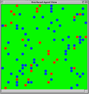
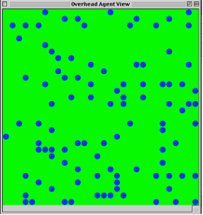
Fig.42: Social Networks Model at t = 14 and t = 30.
To add the social networks visualization to the model, we simply add the following line of code to the createGraphicViews() method in the CoordinationGame class.
public void createGraphicViews() {
overheadView.setDrawNetwork(true);
}
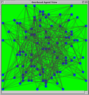
Fig.43: View showing social network ties
There are many interesting permutations of the above social networks model. We can change the interaction networks so that agents play the coordination game with their friends networks and imitate their local neighbors, or we can make the friendship (imitation) relations symmetric. Each of these changes can dramatically alter the dynamics of the model. The basic lesson from network models is that patterns of behavior diffuse much faster through disperse social networks but do not exhibit the discreet spatial patterns that are the hallmark of local interaction models.
In addition to the set() and get() calls for Networks, there are also set() and get() calls for local neighborhoods (setNeighbors() and getNeighbors()). Using these methods actually changes the topology of the lattice so as to make neighbors, in the local, von Neumann sense of neighborhoods, randomly distributed around the graph. In point of fact, setting the neighborhood for an agent and setting a network for an agent can be behaviorally equivalent. However, computationally, they are very different since the former allows an agent to use the Cell and Scape methods such as getNeighbors() and PLAY_RANDOM_NEIGHBOR, to interact with cells that are not spatially related to it. As in the friends network model, we can write analogous methods to perform these operations in a network, but the underlying machinery of the local neighborhoods is unchanged, so the Cell and Scape methods with still refer to the local neighborhood. Setting the Neighborhoods on a scape is tantamount to actually rearranging the geometry of the interactions. Setting a network simply ignores the neighborhood in favor of interacting with a different network of agents.
This concludes the Ascape tutorial. At this point you should be able to develop basic Ascape models, consulting the API documentation for information about how to use functionalities not covered in the tutorial. The basic point to keep in mind while developing in Ascape is that every scape controls the activation and behavior of its member agents. The members of the root scape are (at the very least) a ‘players’ scape and a scape graph. These two ‘agents’ are activated by the root scape’s ITERATE rule. Then, each of these scapes activate their own agents with their own sets of rules. In some cases, the agents activated by the ‘players’ scape, or by some other scape, will be other scapes that hold different agents, and these agents will be told what to do directly by their parent scapes. Thus, collections of agents can interact as agents, and then tell their member agents to perform yet other rules. The possibilities are vast for developing models of societies, and of complex interacting agents.